Determining RAID block size and starting sector, a simple example

Let's walk through the detection of RAID block size and start sector on a simple example. I originally used my Klennet RAID Viewer, but it is now discontinued. However, the functionality is now integrated into Klennet Recovery and is available in the evaluation version. The view is also pretty similar, and the same reasoning and logic apply. I also assume you know at least what RAID is and the well-known RAID levels, RAID0 and RAID5.

The screenshots come from a five-drive set consisting of a four-drive RAID0 and one drive unrelated to the array. There are a few things to keep in mind regarding the choice of disk set:

• RAID level does not matter for this process. While RAIDs with striped parity (RAID5, RAID6, and their derivatives) provide sharper signals, the difference is insignificant.
• Missing drives do not matter. All drives in RAID share the same block size, and missing one or even two drives is not a problem.
• Mixing two different RAIDs in a single scan complicates matters. You can catch it, but it is no fun.

1. Default view

This is the first thing you see when you select the drives and start the analysis. The picture may take a couple of minutes to stabilize, but you can start working on it as soon as you see clearly defined signals. There is no need to wait until the entire disk set is scanned.

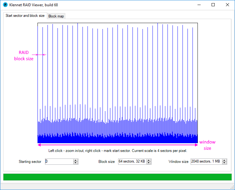
Block size and starting sector view with default settings.

The chart shows the block's probability of starting at a given position on the disk. Higher signals indicate a higher probability. The distance between two "block start" lines indicates RAID block size.

Block size is the size of the RAID block; it is also known as stripe block size or stripe size. The latter term is to be avoided, though (see the very bottom of this page for details). The block size is measured either in sectors or in kilobytes.

Window size is the number of sectors sampled. This setting controls the width of the screen (in sectors).

1. Window size should be larger than the block size; otherwise, you will not be able to see the repeated pattern of block starts and thus will not be able to determine the block size.
2. If the window size is too large, the image will be cluttered (as shown in the example above).

So, the first step is to drop the window size down for a clearer view. Block sizes and window sizes are all powers of two, so each change of block size or window size changes it by a factor of two in the direction you specify.

2. Smaller window size

This is the same view but at a smaller window size, showing eight blocks (eight high signals). This view is already workable, but I prefer one step lower. Red markers (barely visible on the bottom) show the current starting sector and block size selection (0/64 sectors), but it is still irrelevant.

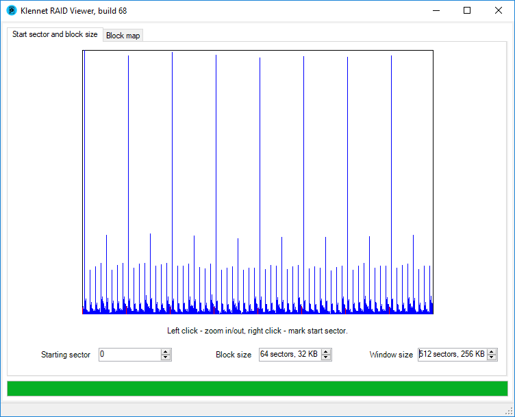
The same view with smaller window size.

So, one more step down on window size.

3. Final display with even smaller window size

This view is a pretty clear. It shows four RAID block starts (high lines), distinct from the background and smaller signals.

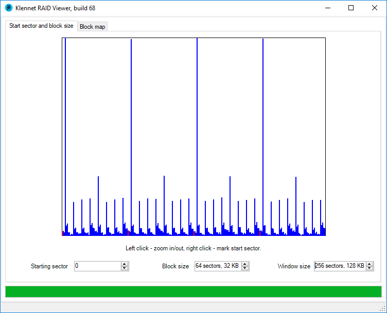
Even smaller window size.

Now, select the block size and starting sector. For starting sector, you can either use an up/down control at the bottom or right-click the highest signal line on the chart. Once starting sector is set, adjust the block size. Your goal is to configure parameters so that all high signal lines are highlighted in red and nothing else is highlighted.

4. Final configuration

So this is what we end up with - the starting sector is 3; the block size is 64 sectors (32 KB).

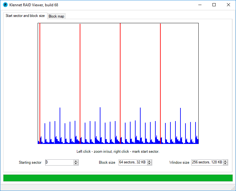
Final configuration with block size and start sector set.

This completes the detection. We now know the correct starting sector and block size for the array and can start deciphering the block map. Block map and disk order analysis for this set is described here if you want to continue with this example.

Additional notes

Lower intensity signals

Typically, there is more than just a RAID block size shown on the chart. Keep in mind that this disk set contains one drive unrelated to the RAID0 array I'm analyzing, and I don't know what is on it. I just took a random drive and stuck it in. With this in mind, let's take a closer look.

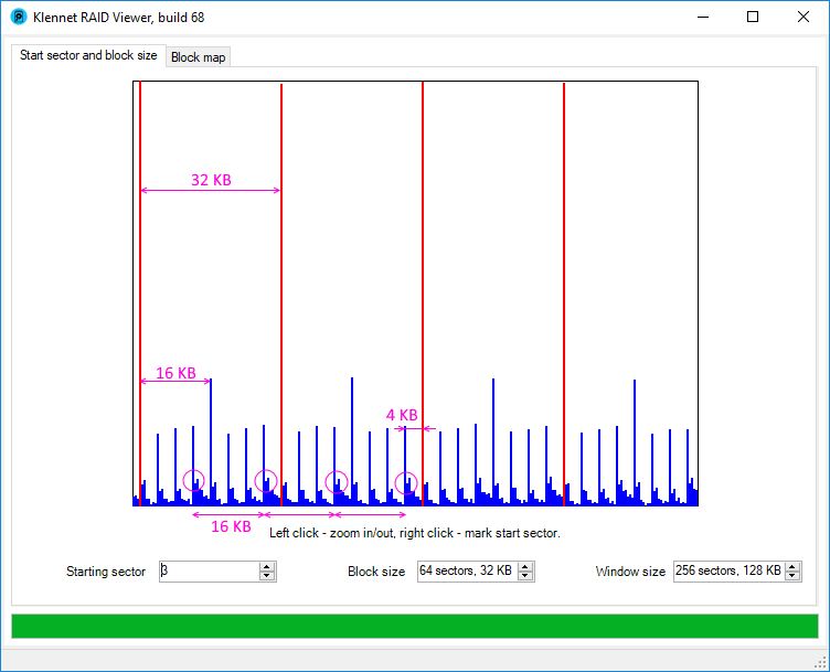
Lower intensity block size signals.

From top to bottom, there are

1. 32 KB primary "start of RAID block" signal, the one we used for the RAID analysis.
2. 16 KB signal matching the cluster size on the non-RAID drive in the set.
3. 4 KB signal matching the cluster size on the RAID itself.
4. Something weird happens every 16 KB, which I can't attribute to anything obvious. While the 16 KB period matches the non-RAID drive cluster size, the start point of this event does not match the start of the 16 KB cluster.

Continue to RAID0 block map analysis

Avoid saying stripe size - it is ambiguous

Consider the following 3-disk RAID0 layout.

Disk 1	Disk 2	Disk 3
1	2	3
4	5	6
7	8	9

• The block size refers to one block (one table cell, green highlight);
• similarly, the stripe block size also refers to one block (the same green highlight);
• however, stripe size may refer either to a single block (green highlight) or an entire row (red highlight).

So, just say block size, which everyone understands.

Back to text

Filed under: RAID.

Created Monday, October 1, 2018

Updated 06 November 2022